Sanctum · a hands-on history & field guide

How Sanctum's Clouds Work

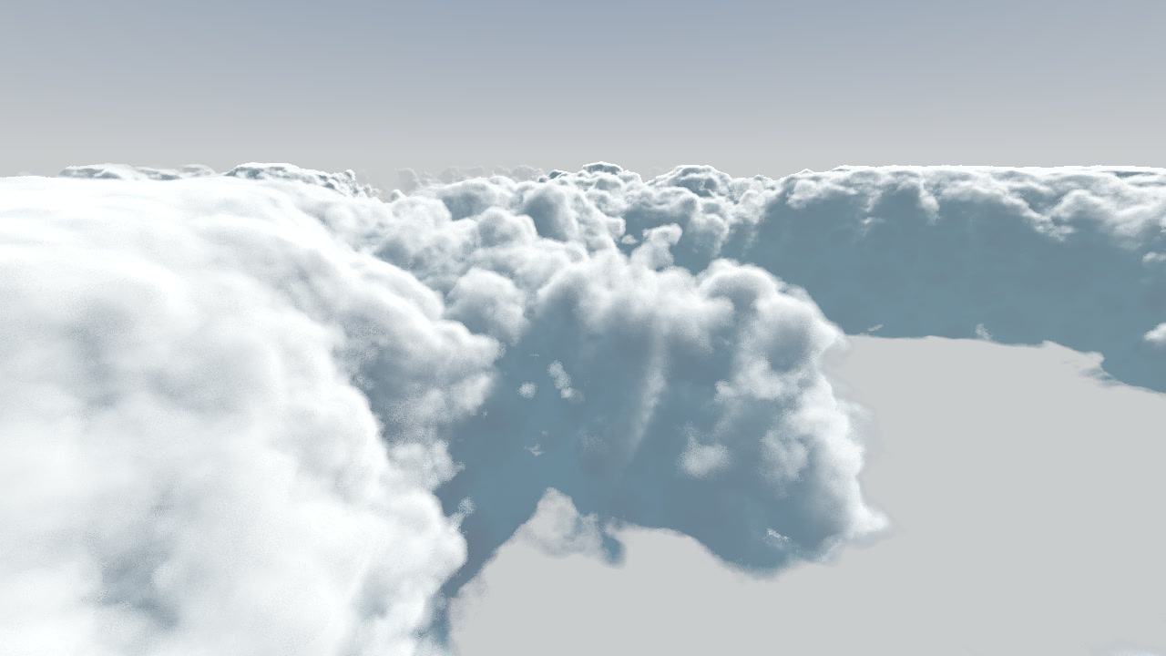
The building blocks of the Sanctum sky — explained in plain English, with the real math, the 3,000-year story behind it, and a live cloud you reshape with your own hands.

Every interactive cloud here is a real GPU render of the Sanctum cloud — the sliders scrub through pre-rendered frames, so it's stunning and runs on anything with no GPU needed.

A towering volumetric cloudscape — the Sanctum production cloud rendered on the GPU
Sanctum's production cloud, rendered on the GPU — a faithful port of Bonkahe's SunshineClouds2. The formulas below are the building blocks of this image — each section is a simplified take on one piece of the pipeline — and you can reshape a live version yourself.
↓ now drag it yourself — scrub the real cloud
Start here. Drag the sun down the sky and watch the Sanctum production cloud relight. As the sun drops, its light must cross far more air — the airmass \(m\) below — which scatters the blue away and leaves the warm sunset you see.
\( m = \dfrac{1}{\sin\,\htmlClass{kx-h}{h}} \)
Sun height
The lineage

Three thousand years in one strip

Not one idea in the Sanctum cloud shader is new. Each formula was cracked by someone solving a completely different problem — measuring starlight, painting a cathedral, photographing a landscape — long before GPUs existed. Real-time clouds borrow from all of them. Here's where the borrowed pieces came from.

~400 BCE
Mozi
pinhole inverts an image
~1021
Ibn al-Haytham
Book of Optics · camera obscura
~1413
Brunelleschi
linear perspective
1435
Alberti
the picture as a window
1733
de Moivre
the bell curve
1760
Lambert
absorption law (after Bouguer 1729)
1852
Beer
adds concentration
1871
Lord Rayleigh
why the sky is blue (1/λ⁴)
1908
Gustav Mie
scattering off bigger particles
1941
Henyey & Greenstein
phase function (for galactic dust)
1950
Chandrasekhar
radiative transfer
1968
Mandelbrot
fractional Brownian motion
1984
Kajiya & Von Herzen
ray-tracing volume densities
1985
Ken Perlin
Perlin noise (Oscar, 1997)
1989
Perlin & Hoffert
hypertexture
1993
Nishita
atmospheric scattering for CG
1996
Worley · Hart
cellular noise · sphere tracing
2002
Reinhard
photographic tone mapping
2010
John Hable
filmic tonemap (Uncharted 2)
2015
Schneider & Vos
Nubis volumetric clouds (HZD)
2016
Hillaire
PB sky & clouds (Frostbite)
~2024
Bonkahe
SunshineClouds2 (open source)
today
Sanctum
Sanctum's port — this page
← scroll sideways → · blue/green = the computer-graphics era · 👆 click any name for their formula
👆 Click any name on the strip above — see the exact formula they contributed and where it lives in the Sanctum cloud.

The big picture

One pixel, five steps

Every dot on your screen is a single ray fired from the camera into the world. That one ray does five things, in order. The rest of the page zooms into each — and tells you who invented it.

01
Pick a sky colour
for the ray's direction — maybe catch the sun
02
March the cloud
step through the volume, gather density & light
03
Add the air
haze & blue between you and the cloud
04
Tonemap
squeeze raw light into a viewable picture
05
Bloom
let the bright bits glow

Step 0 · the camera

How a pixel becomes a ray

The camera sits at one point. Each pixel looks in a slightly different direction — centre dead ahead, edges tilting outward. How far they tilt is the field of view. One line:

\[ \mathbf{dir}=\text{normalize}\Big(\mathbf{forward}+x\,\tan(\tfrac{fov}{2})\,\text{aspect}\,\mathbf{right}+y\,\tan(\tfrac{fov}{2})\,\mathbf{up}\Big) \]
▸ drag the field of view — watch the rays fan out
▸ the camera obscura — why a pinhole flips the image (Mozi, ~400 BCE)
Every point of the world maps to one straight ray through the aperture. Top lands low, bottom lands high — so the image inverts. That single fact is perspective projection.
📜 Where it came from — the oldest math in the renderer

The "one point → one ray" idea is ancient. Around 400 BCE the Chinese philosopher Mozi recorded that light from a person's feet enters a pinhole and lands high while light from the head lands low — so the image flips. Aristotle puzzled over why sunlight through a square hole casts a round spot (a pinhole image of the Sun). The decisive account came around 1021 from Ibn al-Haytham (Alhazen) in his Book of Optics — written, by tradition, while feigning madness to escape an impossible commission to dam the Nile. Renaissance painters then made it constructible: Brunelleschi (~1413) with a peephole-and-mirror demo, and Alberti (1435) framing the picture as "an open window." The GPU's tan(fov/2) is the same idea Alberti pictured, written as trigonometry.

Mozi · ~400 BCEIbn al-Haytham · ~1021Brunelleschi · ~1413Alberti · 1435
“I draw a rectangle… which I regard as an open window through which the subject to be painted is seen.”— Leon Battista Alberti, On Painting (1435)

Step 1 · the backdrop

The sky — two colours and a sun

Before any cloud, the ray gets a sky colour: a blend between a top and a horizon colour, mixed by how high the ray points. The 4th-power curve keeps blue across the dome and crushes the pale horizon into a thin band.

(You already dragged the sun across this cloud up in the hero — that's this exact \(\mathbf{sky}=\text{mix}\big(\text{top},\text{horizon},(1-t)^4\big)\) at work.) The blend curve is what shapes it:

▸ the blend curve \((1-t)^n\)
▸ the sun falloff \(\cos^{p}\theta\) — how tight is the glow?

The colour-space bug that made everything white a real mistake

Sky colours are authored in sRGB (your monitor's space); lighting math must run in linear light. We first fed raw sRGB numbers in as if linear — and the whole scene went 60–90 luma too bright, an "ungodly bright" white-out. The fix is the sRGB→linear decode \(\left(\tfrac{c+0.055}{1.055}\right)^{2.4}\).

📜 Where it came from — a fortunate accident of old TVs

A cathode-ray tube never turned voltage into proportional brightness — its light rose as voltage to the power ~2.5. A nuisance, but lucky: human lightness perception is roughly the inverse of that curve, so "gamma space" also packs detail where the eye is most sensitive. In 1996 HP & Microsoft codified it as sRGB (IEC 61966-2-1, 1999). The catch: sRGB values are not light, so we linearize on read, shade, then re-encode — skip it and blends come out wrong (the white-out).

CRT gamma · TV eraPoynton · Gamma FAQsRGB · HP & Microsoft 1996
“Through an amazing coincidence, vision's response to intensity is effectively the inverse of a CRT's nonlinearity.”— Charles Poynton, Gamma FAQ

Step 2a · the raw material

The noise library — clouds out of static

Cloud shape comes from noise — random-but-smooth patterns, sampled at different scales and stacked. Two famous noises do the work, and they fix each other's weaknesses.

▸ live noise — Perlin is too round, Worley too broken; combined they make cloud
Perlin (fBm)
soft, connected — but blobby
Worley (cellular)
lumpy — but fragmented
Perlin–Worley
Worley erodes Perlin → cloud!
▸ octaves of 1-D noise summing into a natural profile
📜 Where it came from — a movie, an Oscar, and a galaxy of dust

Ken Perlin invented his noise around 1982–83 at MAGI while working on Disney's TRON, frustrated CGI looked too "machine-perfect." He published it in 1985 and won a 1997 Academy Award. The complement came from Steven Worley in 1996: cellular noise, built from distance to scattered points, which reads as organic. Summing octaves traces to Mandelbrot's fractals (his assistant Musgrave brought it to graphics). Decades later Andrew Schneider at Guerrilla combined them for Horizon Zero Dawn — invert Worley to erode Perlin — a recipe Sanctum's renderer follows.

Perlin · 1985 · Oscar 1997Mandelbrot · fractalsWorley · 1996Schneider · 2015
“Movies look better now, and I guess that makes me a good American.”— Ken Perlin, on his Academy Award

Step 2b · shaping the cloud

Density — how much cloud is here?

One function answers "how solid is the cloud at this point?" (0–1), blending the noise through a few dials. Here are the big three, each driving the real cloud.

Coverage — the master "how cloudy" dial

Coverage — how much of the sky fills with cloud. Defined as a "water level" the noise must rise above. Means: raise it and more noise becomes cloud — clear → scattered → overcast.
\( d=\text{noise}-(1-\htmlClass{kx-cov}{\text{cov}}) \)
Coverage
▸ the coverage "water level" over a noise field (the math view)

Sharpness & density — wispy vs firm, thin vs thick

Sharpness \(p\) — how crisp vs soft the cloud is. Defined as a power on the density. Means: low values puff it into soft billows; high values thin it to wispy haze.
\( d \to d^{\,\htmlClass{kx-p}{p}} \)
Sharpness

The real cloud also uses remap (carving one shape out of another) and smoothstep (soft edges instead of hard cutoffs) — the math views:

▸ remap — slide the floor, watch the body erode
▸ hard step vs linear vs smoothstep vs smootherstep
A hard cutoff aliases into jagged rims; the smooth S-curve \(3t^2-2t^3\) feathers cloud edges. From Hermite; Perlin used it as his noise fade.

Step 2c · walking the volume

The raymarch — sampling along the ray

We walk forward in steps, asking "how much cloud?" and adding it up. The number of steps is the quality dial — and you can see it directly:

REAL GPU RENDER
Density silhouette vs fully lit in the real production cloud
◀ what the march finds (density only)+ the lighting below ▶
The Sanctum production cloud: the raw density the raymarch accumulates (left) vs the same density once it's lit (right).
↓ now drive the step count yourself, live (watch it band, then smooth)
Steps — how many samples we take along each ray. Means: too few and the cloud bands into ugly slices; more steps melt it smooth — but every step costs time. The quality-vs-speed tradeoff every real-time renderer fights.
\( \Delta=\dfrac{\text{ray length}}{\htmlClass{kx-N}{N}\ \text{steps}} \)
Steps

But what is each step actually doing? Watch one ray creep in — it peeks at the cloud bit by bit and adds up what it finds:

▸ One ray, marching in step by step — peek, add up, stop when solid (press ▶ replay)
How to read it: your eye (left) creeps along its line of sight in little steps. At each dot it asks "how much cloud is right here?" — orange = inside the cloud, so it adds to the total; faint grey = clear air, nothing to add. The instant the total reads solid, it stops — you can't see past a solid cloud, so looking further (the dashed part) would be wasted work. Thicker cloud → it goes solid sooner; more steps → finer adding-up → the smoother result you dialed just above.
📜 Where it came from — clouds enter the ray tracer (1984)

By 1984 ray tracing had no answer for participating media — clouds, fog, smoke. James Kajiya & Brian Von Herzen (Caltech) reframed it in radiative-transfer physics: store density on a grid, step a ray through it accumulating light. In 1989 Perlin & Hoffert's "Hypertexture" made an object's shape a noise density marched in 3-D — a cloud is exactly that. In 1996 John Hart's "sphere tracing" gave the leap-by-distance trick behind Shadertoy. Sanctum's cloud march builds directly on this.

Kajiya & Von Herzen · 1984Perlin & Hoffert · 1989John Hart · 1996
“Hypertexture exists within an intermediate region between object and not-object.”— Perlin & Hoffert, Hypertexture (1989)

Step 2d · the light

Lighting — what makes a cloud look real

Where a grey blob becomes a sunlit cloud. Four pieces of physics — and you can drive the three biggest.

1 · Beer's Law — bright edges, dark cores

REAL GPU RENDER
A fully lit cloud in the real production render
Beer's-law self-shadow in the Sanctum production cloud — bright sunlit rims, deep dark cores, the soft falloff between. (Real cumulus cores glow grey, because light bounces many times inside them; true multiple scattering is too slow in real time, so Sanctum fakes the look with Beer's-law absorption plus an ambient term — a fast stand-in, not a simulation of the light bouncing around.)

Absorption \(k\) — how fast cloud swallows light, the rate in \(T=e^{-kx}\). High \(k\) = dark dense cores; low \(k\) = thin and translucent. ↓ drag \(k\) on the live curve below and watch the survival rate plunge.

▸ Beer's Law \(e^{-kx}\) — the math view
📜 Where it came from — three people, 123 years, the wrong name

In 1729 Pierre Bouguer — measuring how much starlight the atmosphere swallows (he clocked the Sun at ~300,000× the Moon) — found light loss is exponential with path: equal slabs each remove the same fraction. Lambert restated it cleanly in 1760 (citing Bouguer) — so his name stuck. August Beer (1852) added that it also scales with concentration. The fairest name, "Bouguer–Lambert–Beer," is the least used.

Bouguer · 1729Lambert · 1760Beer · 1852

2 · Henyey–Greenstein — the silver lining

Anisotropy \(g\) — how strongly light keeps going forward through droplets. Means: turn it up and the sun-facing edge lights up with a bright silver rim.
\( \text{HG}=\dfrac{1-\htmlClass{kx-g}{g}^2}{4\pi\,(1+\htmlClass{kx-g}{g}^2-2\,\htmlClass{kx-g}{g}\cos\theta)^{3/2}} \)
Anisotropy g
▸ scattering lobes (polar) — sun from the right; reach = brightness that way
Henyey–GreensteinRayleigh (air)Mie-like (haze)
📜 Where it came from — a formula for starlight in interstellar dust

Louis Henyey & Jesse Greenstein — two astronomers in their early 30s — published this in 1941 to model the glow of diffuse galactic light: starlight scattered by dust between the stars. Real scattering theory was too costly, so they captured the forward-peaked shape with one number, \(g\). That cheap, good-enough trade is exactly why real-time graphics adopted it for clouds, fog, smoke and skin: it captures the forward-peaked shape of droplet scattering with a single knob — close enough to look right, not a true model of how light bends around a droplet. The broader framework came from Chandrasekhar's Radiative Transfer (1950).

Henyey & Greenstein · 1941Chandrasekhar · 1950 · Nobel 1983

3 · The moving sun (& the warm point light)

The same sun you dragged across the cloud in the hero is its key light — low for dramatic, reddened side-lighting; high for bright noon. The sun is white; a separate orange point light at \(\hat{\mathbf{s}}=(\cos e\sin a,\ \sin e,\ \cos e\cos a)\) warms the towers from within.


Step 3 · the air

Atmospherics — depth and the blue of the sky

Between you and a far cloud are kilometres of air that scatter light. The nearer-vs-farther fade is aerial perspective — and it's what gives a flat scene depth:

REAL GPU RENDER
Atmosphere off vs on in the real production cloud and Godot
Godot (target)port — atmosphere OFFport — atmosphere ON
The real production cloud with atmosphere off (flat, pasted-on) vs on (distant cloud recedes into haze — depth).
↓ now drive the haze yourself, live
Aerial perspective — how much distant cloud fades into the hazy air. Means: at 0 the far clouds stay crisp and flat; turn it up and they melt into the blue horizon, and the sky gains depth.
\( \text{haze}=1-e^{-\htmlClass{kx-haze}{\sigma}\,d} \)
Aerial haze
▸ scattering strength across colour — the main reason the daytime sky is blue
Heads up: Sanctum's sky doesn't actually simulate this — it fakes the result with a tuned two-colour gradient that's far faster. The \(1/\lambda^4\) law is just why the colour it's aiming for is blue in the first place.
📜 Where it came from — and the man who got it wrong first

In 1869 John Tyndall saw a light beam through haze glow blue from the side, red from the end — but blamed dust. In 1871 Lord Rayleigh supplied the math: scattering goes as \(1/\lambda^4\), so blue scatters several times more than red (≈4× with real atmospheric numbers) — no dust needed (confirmed to be air molecules around 1899). Larger particles differ: Gustav Mie (1908) solved scattering off any-size spheres — forward-directed and colour-blind, which is why clouds and haze look white. The graphics lineage: Nishita (1993) → Preetham (1999) → Bruneton (2008) → Hillaire (2016).

Tyndall · 1869 (wrong cause)Rayleigh · 1871Mie · 1908Nishita · 1993
“In all cases… the cloud formed at the commencement, when the precipitated particles are sufficiently fine, is blue.”— John Tyndall, 1869

Step 4 · making it viewable

Tonemap — squeezing HDR light into a picture

Lighting produces values past 1.0 (the sun, sunlit tops). A monitor maxes at 1.0, so naive output clips to white. The filmic curve rolls highlights off like film instead:

Exposure — how much light we feed the film curve, \(\text{out}=f_{\text{filmic}}(\text{light}\times\text{exposure})\). Push it up and a naive renderer blows the sunlit tops to flat white; the filmic curve rolls them off. ↓ drag exposure on the live curve below and watch the naive (red) line clip while the filmic (orange) one keeps detail.

▸ filmic curve vs naive clipping — the math view
📜 Where it came from — a 130-year-old photographic curve

In 1890 Hurter & Driffield plotted film density against the log of exposure — the S-curve with a gentle toe and shoulder, so film never abruptly clips. Reinhard (2002) brought it to digital (extending Ansel Adams's Zone System); John Hable fit a real-time version for Uncharted 2 (2010) — the curve Sanctum's tonemap descends from.

Hurter & Driffield · 1890Reinhard · 2002Hable · 2010

Step 5 · the glow

Bloom — letting the bright bits bleed

Real lenses — and your own eyes — bleed light outward from very bright areas. We copy just the bits above a brightness threshold, blur them (a Gaussian blur), and add that glow back on top:

REAL GPU RENDER
Bloom off vs on in the real production cloud
◀ bloom OFFbloom ON ▶
The Sanctum production cloud — in production bloom is kept deliberately subtle (so the off/on is faint by design). Drag the slider below to see what it actually does, pushed well past production.
↓ dial the glow yourself — applied live to a real bloom-off frame
Bloom — copy the brightest bits, blur them, add them back as a glow. Means: at 0 the render is crisp; turn it up and the bright cloud tops bleed a soft halo — like a lens flaring, or squinting at the sun.
\( \text{out}=\text{colour}+\htmlClass{kx-bi}{\text{intensity}}\times\text{blur}\big(\max(\text{colour}-\text{thresh},0)\big) \)
Glow

Bloom — \(\max(\text{colour}-\text{thresh},0)\to\text{blur}\to\text{add}\). Only the bright cloud tops cross the threshold, so the glow lands on the edges without washing out the rest.

📜 Where it came from — a bell curve Gauss didn't discover

The bell curve was written by de Moivre in 1733; Gauss earned the name in 1809 from error analysis (a textbook "Stigler's Law"). Its graphics superpower is separability — a 2-D blur factorizes into a horizontal then vertical pass, \(O(k^2)\to O(k)\) — which is why it dominates GPU blurs and bloom (in games since Riven, 1997).

de Moivre · 1733Gauss · 1809bloom · Riven 1997

The fourth dimension

Animation — making the sky breathe

Each noise octave drifts with the wind at its own speed, so the clouds evolve rather than slide. Here it is in the Sanctum production sky — churning in place, and flown through:

REAL GPU RENDER
Time-lapse of the real cloud evolving
Fixed camera, time-lapsed — the real cloud churns and boils in place as each noise octave drifts.

Animation — \(\text{pos}\mathrel{+}=\text{wind}\times\text{speed}\times dt\). Each octave drifts at its own speed, so the cloud churns and evolves rather than sliding past — the schematic below shows why.
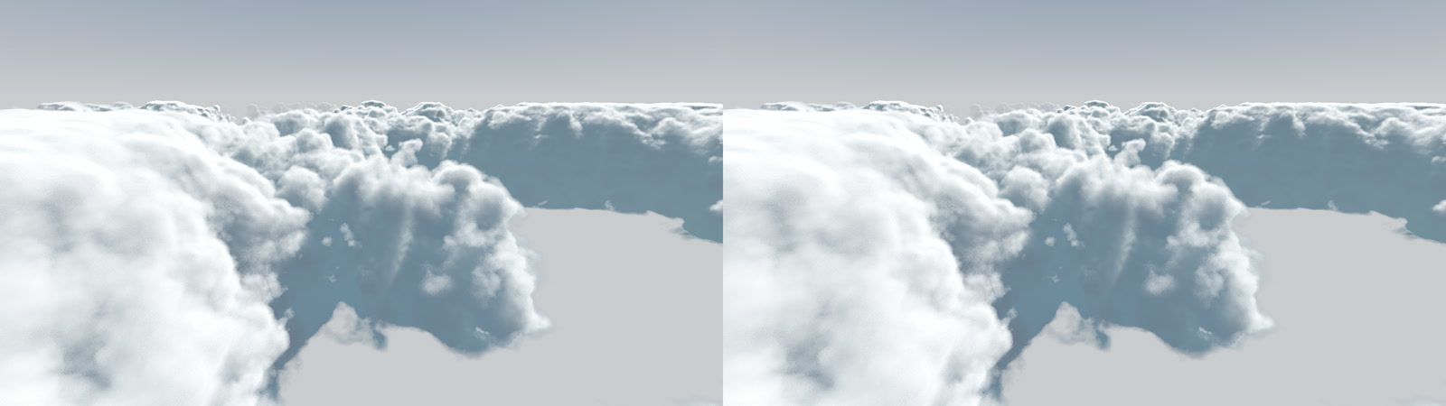
▸ four layers, four speeds — why differential motion reads as "evolving"

The receipt

Is the real thing faithful? — the Sanctum port vs the engine

The cloud you've been dragging is no stand-in — those are real frames from the Sanctum production renderer, a full GPU raymarcher, pre-rendered so the page stays light (only the little math diagrams are drawn live in your browser). And that renderer is itself a faithful port of Bonkahe's open-source Godot shader — so to check the port against the original, the same camera is rendered in both engines and compared side-by-side on the GPU:

Godot vs the Sanctum port, same camera, in motion
GODOT — the real engine (target)SANCTUM PRODUCTION PORT — WebGL ▶
Same vantage, in motion. Recipe and lighting match closely; the one known difference is the noise implementation (baked Worley vs live FastNoiseLite), so individual cloud shapes land in slightly different places.

The whole machine, in one breath

Sky gradient → multi-octave Perlin–Worley density → coverage & remap carving → adaptive raymarch → Beer's-law self-shadow + Henyey–Greenstein rim + ambient + sun → aerial perspective → filmic tonemap → bloom → wind animation.

Every layer is one small, checkable formula — most a century or more old — stacked on the last. You just dragged the main ones.

real GPU framesscrubbed, not recomputedruns on any devicefaithful open-source port

Sanctum vs the original

A faithful port — and what's genuinely Sanctum's

Straight answer: the cloud recipe isn't Sanctum's to claim. It's a faithful port of Bonkahe's open-source SunshineClouds2 (Godot, MIT) — every constant matches Bonkahe's scene, checked against the real engine. That was the point: port it honestly and prove it works. What's Sanctum's is the engineering that got those clouds running — true to the original look — somewhere they were never built to run:

① A compute shader, rebuilt as a web raymarch

Bonkahe's clouds are a Godot/Vulkan compute shader. The Sanctum version is a WebGL2 fragment raymarch — a genuinely different architecture (explicit textureLod, per-ray LOD-scaled marching, no implicit derivatives) to run the same math in a browser.

② Making a Vulkan shader behave on the web

Vulkan tolerates things WebGL/ANGLE don't. Sanctum found and fixed four classes of bug that turned the clouds into NaN-black on Direct3D — a reversed-edge smoothstep, a 0/0 in remap, undefined texture LOD in a divergent loop — plus the catch that ANGLE's fast-math silently eats isnan guards, so bad values must die at the source.

③ It runs on anything — no Godot

Bonkahe's version needs the Godot engine installed. The Sanctum port is a single WebGL2 page: the same clouds on a phone, in a browser, no install — which is the whole reason Sanctum, a three.js MMO heading to Steam, can actually use them.

④ Bonkahe's exact data, re-baked

Sanctum bakes Bonkahe's Godot noise resources into RGBA8 3-D volumes, so the inputs stay Bonkahe's, not an approximation. (The one real visual difference: Bonkahe animates FastNoiseLite; Sanctum marches baked Worley — same recipe, shapes land in different places.)

⑤ Checked against the engine, not just asserted

Sanctum built a Godot ground-truth harness that renders Bonkahe's actual engine, then put the same camera side-by-side in both on the GPU. Recipe and constants match, and the look lines up closely (that's the comparison above) — a close visual match, not a pixel-identical one.

⑥ Where it's heading: a living world

The port proved Bonkahe's clouds work in three.js. Next they get Sanctum's day-night sun-and-moon and world systems driving them — that integration is Sanctum's to build.

So: the cloud math is Bonkahe's, ported faithfully and checked side-by-side against Bonkahe's engine. What Sanctum built is the bridge that makes it run as an MMO using three.js.


Sources & further reading

Every historical claim was researched against primary/reputable sources; where accounts conflict the page hedges. Highlights:

Portrait credits — real likenesses via Wikimedia Commons / Wikipedia. Public domain: Brunelleschi, de Moivre, Lambert, Rayleigh; CC0: Alberti. Creative Commons (attribution): Mie (CC BY-SA 3.0 · ThomasHB4), Chandrasekhar (AIP Emilio Segrè Visual Archives), Mandelbrot (CC BY 2.0 · Steve Jurvetson), Ken Perlin (CC BY 2.5 · Ambuj Saxena), Nishita (CC BY 4.0). Figures with no authentic likeness — and every two-person entry — use a typeset medallion. Source links also in people-meta.json.

Built for Sanctum · the interactive sliders scrub pre-rendered frames of the real production cloud and recompute small illustrative formulas in your browser — no heavy GPU needed (see ISOLATION.md). All beauty imagery is the real GPU render.